Case Study: 10x CouchDB Performance Gains for a AAA Game Launch posted Tuesday, March 4, 2025 by The Neighbourhoodie Team

All software benchmarks and claims of performance are carefully crafted lies and this write-up is no different. Instead of giving you a quick “do steps one, two, three for a magic speedup”, we aim to explain how we arrived at the changes we made and how we rigorously tested those changes to make sure we understand their impact.

All this to give you the tools to follow the process yourself, at the end of which, you might come to very different conclusions that are valid for your particular situation which is very likely different from what our customer was dealing with.

If you need help with your CouchDB, Erlang, or just regular Unix networking performance, book a call today.

Hold on to your hats and get ready for a journey of performance discovery! We will learn about CouchDB and Erlang internals, performance tooling and how to find the next bottleneck in your CouchDB cluster setup.

• The Ask
• The Benchmark
• The CouchDB Situation
• Analysis Part One: Network Throughput
  • Read a document
  • Read a view request
  • Interlude: How to Benchmark
• Analysis Part Two: Input/Output
  • A Brief Erlang Detour: Processes
• Analysis Part Three: HTTP Request Tracing
• Analysis Part Four: TCP Accept
• Analysis Part Five: CPU Utilisation & Process Scheduling
• Analysis Part Six: Erlang Network Messaging
• Conclusion

The Ask#

Our CouchDB Support customer has been using CouchDB for over ten years as the backend for a AAA sports game and they were getting ready to launch their newest edition a few weeks away from when they contacted us.

Their setup is a six-node CouchDB cluster hosted on AWS EC2, 192 cores each, 768 GB RAM, NVME storage, the works. They set up one cluster each for each iteration of the game, so they could make some informed decisions about hardware sizing versus expected performance numbers.

That said, with roughly 3x larger nodes (in terms of CPU and RAM) as well as a whole additional node (the previous game is running on a five-node cluster), their benchmark showed a mere 50% increase in requests per second (req/s). Nowhere near the 3x + 1 node.

Quick aside: sometimes you come across performance discussions and the metric used is requests per minute, usually to make the numbers look more impressive. Don’t let that fool you, requests per second is where it’s at.

In addition to the meagre performance improvement, the customer also noticed a 10x increase in request latency while running the benchmark. That’s neither expected nor desirable.

While their benchmark reflected a worst case in total number of requests and request concurrency, and the median case was handled just fine by the new cluster, the results were not satisfactory so we were called in to see:

1. Was there more req/s to be had?
2. Can we improve on the 10x the latency spike under load?

With those goals in sight, we set to work.

The Benchmark#

First, we need to discuss the benchmark, because as benchmarks go, it was not a very good benchmark. No shade to the customer for making a “bad“ benchmark, we support whatever gets the job done.

But how exactly did we (and the customer themselves) conclude the benchmark was bad? Well, they tested things in a way that played against the strengths of CouchDB. They knew their actual applications would never organically behave this way, but if we could make CouchDB work well despite the benchmark trying very hard to not play ball, the customer was certain their application would work fine.

So this wasn’t a kind of benchmark that was trying to most adequately model the client application behaviour — those are usually complicated to create and orchestrate — instead, this benchmark existed to establish a worst-case baseline while only taking a few minutes to create vs. the days and weeks that a more accurate benchmark would take to produce.

The benchmark consisted of nine invocations of the trusty old ab (“Apache Bench”) tool. It allows you to send a single type of HTTP request over and over again with a defined concurrency. This is very brute-force, but ab has existed since the 1990s and just does this simple job very well.

Aside: these days, a lot more and better tooling exists, but few are as simple as ab, which is why this was an okay choice for the worst-case baseline benchmark.

The benchmark instructed to launch multiple instances of ab:

• 4x each retrieving a specific document from a database,
• 5x retrieving the first result row of a view in one of 4 databases.

Each instance of ab would make its same request one million times at a concurrency of 300.

And here you can directly see why this is a “bad” benchmark: in real-life, the application would never request the same document a million times with 300 concurrent requests. If a piece of data would have this read frequency, it would live in an in-memory cache or even just be cached in the application server heap.

And one final note: this is not a scientific benchmark where we calculate the statistical significance of the results we are seeing. We are not trying to establish the theoretical and practical limit of CouchDB itself, but we want to find the worst-case scenario limits of this specific setup. Everyone involved was satisfied with the methodology. We just want to note that this type of thing can be done with a lot more rigor that was not needed here.

For now, enough about the benchmark, let’s look at the CouchDB side of things.

The CouchDB Situation#

Before we can dive into the CouchDB setup, we need to explain some CouchDB internals, namely database sharding: each database in the CouchDB URL space…

• /db1
• /db2
• …

consists of one or more shards. A shard is an individual database file that stores its data in an append-only B+tree, used via a single file descriptor. Writes are serialised and reads can occur concurrently (although current developments in the CouchDB project examine whether there is an improvement to be had).

By default, CouchDB splits databases into 2 shards and all data is equally shared among these. As a best practice, CouchDB shards should not exceed 10GB of data or 10M documents (whichever gets there first) to keep performance and maintainability under control. Once you reach these sizes, you can engage CouchDB’s shard splitting feature as often as you need it.

Alternatively, if you know you’ll be reaching your target sizes quickly, you can choose a higher sharding level upfront and never bother with splitting. This is what the customer has chosen in the past and has chosen it again for this iteration, and their shard level (or q) is 60. From this you can deduce, they are expecting a lot of data.

Sharding a database has multiple effects:

1. You can store more data that fits on a single node by distributing each shard onto a different node.
2. You can increase parallel read and write performance as each shard is limited to the throughput of a single file descriptor and all writes are limited to the throughput of a single CPU core. More shards means more CPU cores can work on more file descriptors in parallel, leading to more throughput overall.
3. The trade-off that enables point 2 is that requests that aggregate data from all distributed shards, like _all_docs, _changes, a view query or a mango query will slow down linearly with the number of shards. Partitioned databases can help with this in some very specific cases. However, the customer could not take advantage of those.

So in general: sharding is good for increased parallel document performance, but can be detrimental to view query performance. And if you remember, the benchmark was doing both.

Analysis Part One: Network Throughput#

When the customer demonstrated the behaviour to us on a video call, our immediate gut reaction was that there was something wrong with the network. Why?

For this we have to go into a little more detail on how CouchDB clustering works.

Any of the nodes in a cluster can receive any request and will try to answer it. Normally, requests arrive via a round-robin load balancer: if a node has the data requested, it will return it, and if not, it will forward the request internally to one or more nodes that do have the data.

This is the first thing to learn: CouchDB has an external HTTP API that listens on post 5984 and an internal network called Erlang Distribution that allows all nodes in the cluster to efficiently talk to each other.

In even more detail, document operations behave differently from view operations:

Read a document#

To read a document (docA, docB) from a cluster, the receiving node will first map the document’s _id onto the shard range it lives on and then send an internal request for all the shards of that range. Did we not mention, each shard range exists on n=3 different nodes for high availability? Now you know. CouchDB will send an internal request to all three shard range copies to retrieve the document, and the first two responses that agree on the result constitute the response. This is called a quorum request. You can learn more about how this works in the CouchDB documentation.

Read a view request#

To read a view request, the receiving node will have to contact each view shard in the cluster, that is every shard range, and retrieve the rows that are relevant and then return an aggregate of those. So while a document operation will result in at most 3 internal requests, a view result requires at least q internal requests, one for each shard.

You might deduce from this that a database with shard level q of 60 creates a lot of internal requests and you would be correct.

With lots of internal requests needed for the benchmark, our instinct led us to networking issues right away.

The customer took this advice and overnight (for us) did some dedicated network benchmarking and noticed immediately that they were throttled at 1 Gb/s, even though the AWS instances should support 25 Gb/s. They quickly determined that since they had started on smaller instance sizes early on in the setup and since migrated to larger ones, the AWS setting for faster networking was not enabled 🎉

After resolving this, the dedicated network benchmarks showed a 25Gb/s link to be available. The CouchDB benchmark showed that the limiting factor now was no longer the network, but the original observation still held.

Aside: CouchDB can be configured to separate external and internal networking onto two separate network interfaces (NICs) and we generally recommend that setup for high-performance installations, but with the network shown not to be a bottleneck, the customer opted to keep a single-NIC setup for now.

With this issue out of the way, we tackled the next candidates for bottlenecks.

Interlude: How to Benchmark#

The aim of benchmarking ultimately is to find a limit of software and hardware for a certain load pattern. A lot of things on the hardware side can contribute to such a limit:

• available CPU cycles
• available RAM
• network latency and throughput

…and our job was to find out when CouchDB would run up against one of these limits and see if we can improve on it. The process is always iterative and continuous. The only way to make a computer go faster is to have it do fewer things. And there are always fewer things to do to achieve the same result until you hit a theoretical limit. In practice, the time and budget available will lead to a “good enough” situation rather than reaching that theoretical limit, but the process is always one of finding the next bottleneck.

Say you eliminated a networking bottleneck like we just did, but the problems still show, naturally there exists a further bottleneck that is likely not the network, but one of the other available computing resources.

So that’s what we were going to cover next.

Analysis Part Two: Input/Output#

Before we started trying to find the next bottleneck, we wanted to learn about how the benchmark affects the system. Since there are two types of requests:

1. concurrent document requests
2. concurrent view requests

We tried each type in isolation and we could quickly deduce that the concurrent document reads basically have no effect whatsoever. This was not too surprising but well worth ruling out. We could now focus on concurrent view requests exclusively, making the whole process a little easier and faster.

A different CouchDB Support issue that we handled at Neighbourhoodie just a few weeks back pointed us to disk IO being the bottleneck. Since we knew how to verify this is the issue quickly now, we did that next.

There are two places you can look for disks being the bottleneck:

1. iowait is a UNIX OS metric that tells you how much the kernel is waiting on a disk to fulfil an operation. If this is consistently high (should be 0-ish) you can tell that your disk cannot keep up with the requests you are sending to it.

   In our case, that wasn’t it. iowait was rising a little during the benchmark, but nowhere near as high to cause an issue.

   If you are using AWS EBS, there is a separate EBS metric that gives you this number for your EBS stores: VolumeQueueLength.

2. If the disk is fast enough, maybe we have a limit on how much data we can send to it. Remember earlier when we explained that a single shard is backed by its own file descriptor? It is possible to exhaust how much traffic can be transferred through one of these, but it’s pretty high, so unlikely to be the issue. But there is more: each shard is managed by a single instance of a couch_file process inside CouchDB.

Now we need to learn about processes in Erlang.

A Brief Erlang Detour: Processes#

Erlang programs are built around processes that are launched, that run and that exit. Processes can launch other processes, processes can observe other processes and processes can send and receive messages from other processes.

Processes behave much like operating system processes in most ways but one: They are lightweight as in you can start millions of them in a second and stop them even faster. They are what make Erlang especially well suited for building programs that can handle many concurrent requests, like CouchDB.

Every process in Erlang has got a message inbox that contains all the messages that other processes send to it in sequence. Each message can only be handled one at a time. So if more messages arrive than can be handled, the message inbox grows.

And one final piece of the puzzle: an Erlang process runs on a scheduler and that scheduler is tied to a single CPU core. So whatever happens inside this process, it can never go faster than a single CPU core.

Back to the analysis: a message sent to a couch_file process could be asking for the contents of the document or a view result row that lives at the file offset O and is L bytes long. Now if there are a lot of requests coming in concurrently, there is a chance that there are more requests coming in than either the CPU, the file descriptor or the disk can handle and the process message queue can grow indefinitely.

We already ruled out the disk with iowait, so what’s next? We can observe the Erlang process message queue in (near) real time!

Much like you can run ssh into a server and list all its processes with ps ax, you can remsh into an Erlang VM and list all its processes with processes(). Running remsh gives you an interactive shell that runs inside the Erlang VM and you can type Erlang code to inspect the system. Since coding all that inspection by hand can be a bit tedious (and error-prone), CouchDB comes with the excellent recon library that simplifies common observation tasks and makes them safe to run in production.

Here is how it looks like when you invoke remsh and run recon commands:

> /opt/couchdb/bin/remsh
Erlang/OTP 25 [erts-13.2.2.11] [source] [64-bit] [smp:14:14] [ds:14:14:10] \
[async-threads:1] [dtrace]

Eshell V13.2.2.11  (abort with ^G)
(couchdb@127.0.0.1)1> recon:proc_window(message_queue_len, 3, 5000).
[{<0.16793.2083>,0,
  [{current_function,{prim_inet,accept0,3}},
   {initial_call,{proc_lib,init_p,5}}]},
 {<0.16788.2083>,0,
  [{current_function,{prim_inet,accept0,3}},
   {initial_call,{proc_lib,init_p,5}}]},
 {<0.16579.2083>,0,
  [{current_function,{prim_inet,accept0,3}},
   {initial_call,{proc_lib,init_p,5}}]}]
(couchdb@127.0.0.1)2> 

While this might look like gibberish to the casual observer, we’re here to explain how to read this.

Anything prior to recon:proc_window(message_queue_len, 3, 5000). is starting the remsh program to log into a running CouchDB instance. It prints some metrics about the Erlang VM like its version, how it was built, how many schedulers are running as well as various other bits and pieces. It ends with a prompt for us to type commands in, like the one at the beginning of this paragraph.

This command invokes the proc_window function on recon module and we are passing in three arguments:

1. message_queue_len the metric we are interested in
2. 3 to return the top three processes with the longest message_queue_len
3. 5000 the sample duration in milliseconds (ms)

With this recon:proc_window() observes the Erlang VM for five seconds and collects all processes’ message_queue_len, sorts them by their respective value, and returns the top three. The result is a list of the form {Pid, MessageQueueLen, Callstack}.

Our sample output here is not very interesting, just processes that are waiting for requests to come in and their inbox is 0. But when we run an ab benchmark similar to the one our customer ran, we can observe a different set of processes in the top three.

(couchdb@127.0.0.1)5> recon:proc_window(message_queue_len, 3, 5000).
[{<0.3.0>,4,
  [{current_function,
       {erts_dirty_process_signal_handler,msg_loop,0}},
   {initial_call,{erts_dirty_process_signal_handler,start,0}}]},
 {<0.20014.2083>,3,
  [{current_function,{prim_file,pread_nif,3}},
   {initial_call,{proc_lib,init_p,5}}]},
 {<0.353.0>,2,
  ['rexi_server_couchdb@127.0.0.1',
   {current_function,{gen_server,loop,7}},
   {initial_call,{proc_lib,init_p,5}}]}]

The first one has a message_queue_len of 4, it is deep inside the Erlang internals, the details of which are not in scope for this discussion (yet). The third one is also out of scope, but we note the message_queue_len of 2.

The second one is more interesting. That’s a process that is also deep inside the Erlang internals, but at a part that is relevant to us: reading files. The prim_file:pread_nif function reads bytes from a file descriptor and its message_queue_len is 3, so there are more bytes requested to be read than this particular process can handle and read requests stack up.

It looks like we found something, great! Unfortunately, this is from a demo setup and doesn’t reflect the customer benchmark well enough to draw conclusions from, this is just to demonstrate how to find processes that might be overwhelmed.

And another unfortunately: a message_queue_len in single digits is totally fine. So while illustrative of how this process works, this particular example does not exhibit any bottlenecks.

Aside: we had to patch the metrics collector the client was using, because it didn’t collect message_queue_length metrics correctly, which is the whole reason why we had to do this in remsh. Our patch has been contributed back to the metrics vendor, so everybody can benefit from it going forward.

And on our customer’s systems, under benchmark, it was much the same. While we did see spikes in the message queues for some processes, they were very short lived and not at volumes that were showing a bottleneck.

So we ruled out networking and disk, the two metrics that comparatively can have the biggest impact on performance as they are the slowest relative to the CPU. In that hierarchy, looking at RAM would be next, but it did not look as though large or lengthy allocations or garbage collection were happening. And CPU utilisation was at 5% of the whole cluster capacity with no one CPU core being maxed out, so we felt we had to understand what was going on a little better.

Analysis Part Three: HTTP Request Tracing#

At this point we went back to look exactly at how we are observing the effects of the benchmark. At the highest level, we found we could show the increased latency best in a call to CouchDB’s _dbs_info endpoint while the rest of the benchmark was running.

It is an endpoint that returns information about all databases, their names, the number of documents inside, file sizes, the lot. Like views, it has to talk to all 60 shards per database to collect this information. It does this for all databases, so understandably, even though it might not return large amounts of data, the work it needs to do to collect that data is not trivial. In addition, those are the same files being used by the benchmark, so we are expecting contention here.

We could observe that when the benchmark was not running, the cluster would take around 400–500ms to produce a full result and send it back as JSON as measured by timeing curl:

> time curl -su user:pass http://127.0.0.1:5984/_dbs_info > /dev/null

real	0m0.497s
user	0m0.008s
sys	0m0.008s

Here we can see that the request took 497ms (~500ms) to complete while using very little other system resources, so we were mainly waiting for IO here.

Now the experienced among you will jump up and shout about the improper use of time. What does that do? Simply: it runs the program you pass to it and then measures how long it took to run. This time includes forking a new operating process for curl. So for very narrow timings, it is not useful, but the overhead is very small when dealing with network operations, even on the same host.

For comparison, see how time ls > /dev/null fares on the developer machine this is written on:

> time ls > /dev/null

real	0m0.004s
user	0m0.001s
sys	0m0.002s

4ms to launch ls and return five directory entries. Not enough to make a significant dent into the ~500ms of our _dbs_info request.

Now, with the benchmark running, our curl to _dbs_info grew taking up to 12 seconds, roughly a 20x slowdown and very much not acceptable for a production setup.

Then we got curious, there are multiple parts inside CouchDB that are responsible for handling a request. The cascade goes like this (brace for jargon, all will be explained):

1. chttpd starts a mochiweb acceptor that receives incoming TCP requests, parses them and hands HTTP requests to chttpd.
2. chttpd routes incoming HTTP requests to fabric which, with the help of rexi , makes the internal cluster requests we have been talking about earlier and collects the results.
3. fabric then talks to the relevant CouchDB subsystem for the particular request, like couch_server for database requests, or couch_index_server for view results, or couch_replicator for initiating replications.
4. Finally, chttpd returns the result(s) it received from the subsystem as JSON.

And we got curious where exactly things got slow. Luckily, the implementation of _dbs_info made that very convenient. It aims to send HTTP response headers as soon as it can after receiving the incoming request, so as not to leave clients waiting, but then it calls into fabric for the data that goes into the response body.

Why is that lucky? Because curl lets us observe these distinct steps without the coarse granularity of time.

With the -v --trace-time options, curl tells us for each line of output when that was received. This is again from a local dev machine just to show the output. As you can see, the timestamps for each line show with microsecond precision what happened when.

> curl -u admin:admin http://127.0.0.1:5984/_dbs_info -v --trace-time
12:09:19.647540 *   Trying 127.0.0.1:5984...
12:09:19.649708 * Connected to 127.0.0.1 (127.0.0.1) port 5984
12:09:19.649758 * Server auth using Basic with user 'admin'
12:09:19.649808 > GET /_dbs_info HTTP/1.1
12:09:19.649808 > Host: 127.0.0.1:5984
12:09:19.649808 > Authorization: Basic YWRtaW46YWRtaW4=
12:09:19.649808 > User-Agent: curl/8.7.1
12:09:19.649808 > Accept: */*
12:09:19.649808 > 
12:09:19.649955 * Request completely sent off
12:09:19.653295 < HTTP/1.1 200 OK
12:09:19.653330 < Cache-Control: must-revalidate
12:09:19.653357 < Content-Type: application/json
12:09:19.653382 < Date: Fri, 07 Feb 2025 11:09:19 GMT
12:09:19.653407 < ETag: "55VZ21K2GFXCUV8ZTDGIB0766"
12:09:19.653433 < Server: CouchDB/3.4.2 (Erlang OTP/25)
12:09:19.653460 < Transfer-Encoding: chunked
12:09:19.653484 < X-Couch-Request-ID: 26578fcf5c
12:09:19.653508 < X-CouchDB-Body-Time: 0
12:09:19.653532 < 
[{"key":"asd","info":{"instance_start_time":"1695218554","db_name":"asd","purge_seq":"0-g1AAAABXeJzLYWBgYMpgTmEQTM4vTc5ISXIwNDLXMwBCwxyQVB4LkGRoAFL_gSArkQGP2kSGpHqIoiwAtOgYRA","update_seq":"0-g1AAAACbeJzLYWBgYMpgTmEQTM4vTc5ISXIwNDLXMwBCwxyQVB4LkGRoAFL_gSArgzmRIRcowJ6cmGiUmmiKTR8e0xIZkupRjDGyMEk1NUjCpiELAAzhKKI","sizes":{"file":16686,"external":0,"active":0},"props":{},"doc_del_count":0,"doc_count":0,"disk_format_version":8,"compact_running":false,"cluster":{"q":2,"n":1,"w":1,"r":1}}}]
12:09:19.654131 * Connection #0 to host 127.0.0.1 left intact

Our first point of interest was the line * Request completely sent off. At that point, CouchDB had fully received the request and was starting to calculate the response headers that were sent shortly after between 12:09:19.653295 and 12:09:19.653508 in the output above. After that, we see how long it took to collect the response body and how long it took to send the body back to curl.

Broken out, the three phases took:

1. receiving the request: 12:09:19.649955 - 12:09:19.647540 = 2415µs or 2.4ms
2. sending the response headers: 12:09:19.653532 - 12:09:19.649955 = 3577µs or 3.5ms
3. sending the response body: 12:09:19.654131 - 12:09:19.653532 = 599µs or 0.5ms.

In our sample case here the body with just a single database was even faster to send than the headers. But on the customer cluster we got these measurements (averaged from multiple runs).

Without the benchmark:

1. receiving the request: ~2ms
2. sending the response headers: ~10ms
3. sending the response body: ~485ms

Most of the time spent in sending the body.

And during the benchmark:

1. receiving the request: ~4ms
2. sending the response headers: ~100ms
3. sending the response body: ~12000ms

Reading the results backwards, the increase in receiving the response body was expected and similar to what time roughly indicated, but the delay in sending request headers and the increase in sending the response headers was surprising.

From this we hypothesised that we were not dealing with a single bottleneck but potentially two:

• one when accepting new requests,
• one when collecting response body data from many shards across the cluster

To validate the hypothesis, we decided to test a different CouchDB endpoint, one that goes through all the steps. But when fetching the data for the response body, it only talks to an in-memory data structure from a single node in the cluster, so it should be extremely fast. This request avoided any disk IO as well as any internal cluster communication.

If we could show that a request to the _config endpoint also had a slowdown when making a request under benchmarking, we could be reasonably sure that we found an additional bottleneck when receiving requests. For this we used time- based measuring again, as it was sufficient to show the difference.

And we found this, without the benchmark:

time curl -su admin:admin http://127.0.0.1:5984/_node/_local/_config > /dev/null

real	0m0.009s
user	0m0.003s
sys	0m0.003s

And with the benchmark running:

time curl -su admin:admin http://127.0.0.1:5984/_node/_local/_config > /dev/null

real	0m0.132s
user	0m0.003s
sys	0m0.003s

Hypothesis confirmed, we were dealing with two bottlenecks. We chose to tackle the bottleneck of accepting requests first.

Analysis Part Four: TCP Accept#

CouchDB uses a library called mochiweb for listening to HTTP requests arriving over a TCP socket. The way this works is CouchDB provides a callback function for handling a request and then tells mochiweb to start listening to a socket and port (or two in case TLS is enabled). The callback function that leads to matching the path of a request against a set of handlers for that specific endpoint.

Since we’re interested in handling connections, we need to look at mochiweb. The customer had these config options set in their CouchDB configuration:

[chttpd]
server_options = [{backlog, 128}, {acceptor_pool_size, 16}]

backlog is an option that is passed to the TCP stack of the operating system and it defines how many connections can queue up on a socket before they are being dropped. This is another inbox-type queue that ideally has very low numbers in practice, but it is a good memory and latency trade-off against dropping connections when a server sees a sudden spike.

As far as we could tell there were no dropped connections. But we wanted to see anyway how many requests were waiting in the backlog when the benchmark ran as it could be that even if the backlog does not overflow, having it constantly be very full might account for our accepting requests bottleneck.

Linux comes with a tool to look at socket statistics (unfortunately) called ss. We used it in a while loop to dump out the current state for the CouchDB port 5984.

The Send-Q column shows our defined backlog config option, Recv-Q changes as requests come in and increases as requests are queued up.

while true; do ss -lti '( sport = 5984 )'; sleep 0.5; done
# we know about `watch`, we prefer the while loop for more flexibility
State     Recv-Q    Send-Q       Local Address:Port        Peer Address:Port   Process
LISTEN    0         128               0.0.0.0:5984            0.0.0.0:*
	 cubic cwnd:10
…

Whatever we tried, we did not get this to show that the 128 queue limit was exceeded. We sometimes saw Recv-Q climb into the 40s to 60s but never for long. We also experimentally tried setting backlog to 256 to make sure our half-second sampling wouldn’t miss anything. But it made no difference on the benchmark and the resulting increased latency behaviour, if anything, it made the memory-only request to _config a little slower.

acceptor_pool_size is a mochiweb setting that defines the number of Erlang processes (remember: lightweight) that handle the accepting of a request. The default of 16 means that 16 new connections can be accepted at any one time. We have not had occasion to change this setting in the past, but since it was related to our problem, we tried increasing it to 32 and we did see a difference.

Quick aside: when making configuration changes to see their effect on a benchmark, we followed these hard earned rules:

1. Change one thing, and one thing only, before testing again. That way you can be sure the thing that you change actually has an effect. If you were to change two or more things, you don’t know if any one of the changes or a combination of two or more changes lead to your new observation. This might sound tedious, especially with longer running benchmarks, but untangling a less disciplined situation will always take longer or lead to unclear results.
2. When you do change a value, make a meaningful change to make sure you see an effect, but also don’t make too big a change as that might cause widely differing behaviour. It is better to increment conservatively and go in a couple of steps rather than doing a big jump. In practice, increments of 2x or 10x (depending on the values) have been found to be useful. We chose 2x over 10x here as doubling the total number, that we never had to change in the past, should show any difference well if it made any, without being widely different when setting it to 160. In other cases, say you want to find the sweet spot for document sizes in CouchDB, 100 bytes, 1k, 10k, 100k and so on are a good sequence of 10x increments. Using 2x to climb that progression will take a while and you can save some time.
3. Find the limits: when you do observe a change, keep going at least one more step to see if things change even more, or if they stabilise around the new number. In our case, we also tried 64 and it didn’t make any difference. If you are doing a 10x progression and you find an inflection point, it might be worth going back to 5x (and a half step in either direction from there) if you want to find a true local optimum.
4. As for your benchmark: make sure to run it multiple times and take average, median, 95th and 99th percentile measurements.
5. Once you have validated that your one change made a difference, undo it and re-measure to see if the effect is reversed and not a random fluke.
6. End of aside.

We made a 2x change to the acceptor_pool_size, set it to 32 and ran the benchmark again. We did our while loop with the socket stats again and noticed slightly higher queue levels than before, but still no exceeding 128.

However, the biggest difference we saw was in the time for requests to be accepted, both _config endpoints that only read from memory as well as the more heavyweight _dbs_info request did increase in accept times. But instead of going from ~10ms to ~100ms, they went from ~10ms to ~12ms.

This is it! We found our next bottleneck! 🎉 We were sending so many concurrent requests (nearly 3000 across all the ab instances) in the benchmark, that the acceptor pool could not keep up. This did not show up in the Erlang message queue measurements because the queueing happens in the operating system’s TCP layer and not inside Erlang.

A 20% higher request accept latency is entirely acceptable at the total number of requests being handled. Well done team and onto the next frontier: the 12s response body latency of _dbs_info.

We reported this back to the CouchDB project and an acceptor_pool_size of 32 is the default from versions 3.4.3 / 3.5.0 onwards.

Analysis Part Five: CPU Utilisation & Process Scheduling#

Next we looked closer at CPU utilisation again. Apart from not maxing out the available CPU cores and not overloading a single CPU core / Erlang scheduler, we didn’t have a good understanding where exactly CPU time was spent just to see if there was another type of bottleneck that wasn’t shown in regular CPU observation (top and Datadog in this case).

Modern Erlang comes with a number of performance profiling utilities and one of them is msacc (microstate accounting). It gives a more detailed view into what the Erlang VM is doing. It is again used via remsh like recon.

Our particular invocation ran for 10 seconds at a time and printed stats of (Erlang) system information.

msacc:start(10000), msacc:print(msacc:stats(), #{system => true}).

The output of the machines under investigation was a bit unwieldy as each scheduler gets an individual utilisation row and the machines started 192 schedulers, one for each CPU core, so we’ll be showing sample output from a smaller machine:

Average thread real-time    :  10000197 us
Accumulated system run-time : 123357711 us
Average scheduler run-time  :   4814134 us

        Thread      aux      check_io      emulator            gc         other          port         sleep     

Stats per thread:
     async( 0)  0.00%( 0.0%)  0.00%( 0.0%)  0.00%( 0.0%)  0.00%( 0.0%)  0.00%( 0.0%)  0.00%( 0.0%)100.00%( 2.1%)
       aux( 1)  1.32%( 0.0%)  1.33%( 0.0%)  0.00%( 0.0%)  0.00%( 0.0%)  0.26%( 0.0%)  0.00%( 0.0%) 97.09%( 2.1%)
dirty_cpu_( 1)  0.00%( 0.0%)  0.00%( 0.0%)  0.00%( 0.0%)  0.00%( 0.0%)  0.00%( 0.0%)  0.00%( 0.0%)100.00%( 2.1%)
dirty_cpu_( 2)  0.00%( 0.0%)  0.00%( 0.0%)  0.00%( 0.0%)  0.00%( 0.0%)  0.00%( 0.0%)  0.00%( 0.0%)100.00%( 2.1%)
dirty_cpu_( 3)  0.00%( 0.0%)  0.00%( 0.0%)  0.00%( 0.0%)  0.00%( 0.0%)  0.00%( 0.0%)  0.00%( 0.0%)100.00%( 2.1%)
dirty_cpu_( 4)  0.00%( 0.0%)  0.00%( 0.0%)  0.00%( 0.0%)  0.00%( 0.0%)  0.00%( 0.0%)  0.00%( 0.0%)100.00%( 2.1%)
dirty_cpu_( 5)  0.00%( 0.0%)  0.00%( 0.0%)  0.00%( 0.0%)  0.00%( 0.0%)  0.00%( 0.0%)  0.00%( 0.0%)100.00%( 2.1%)
dirty_cpu_( 6)  0.00%( 0.0%)  0.00%( 0.0%)  0.00%( 0.0%)  0.00%( 0.0%)  0.00%( 0.0%)  0.00%( 0.0%)100.00%( 2.1%)
dirty_cpu_( 7)  0.00%( 0.0%)  0.00%( 0.0%)  0.00%( 0.0%)  0.00%( 0.0%)  0.00%( 0.0%)  0.00%( 0.0%)100.00%( 2.1%)
dirty_cpu_( 8)  0.00%( 0.0%)  0.00%( 0.0%)  0.00%( 0.0%)  0.00%( 0.0%)  0.00%( 0.0%)  0.00%( 0.0%)100.00%( 2.1%)
dirty_cpu_( 9)  0.00%( 0.0%)  0.00%( 0.0%)  0.00%( 0.0%)  0.00%( 0.0%)  0.00%( 0.0%)  0.00%( 0.0%)100.00%( 2.1%)
dirty_cpu_(10)  0.00%( 0.0%)  0.00%( 0.0%)  0.00%( 0.0%)  0.00%( 0.0%)  0.00%( 0.0%)  0.00%( 0.0%)100.00%( 2.1%)
dirty_cpu_(11)  0.00%( 0.0%)  0.00%( 0.0%)  0.00%( 0.0%)  0.00%( 0.0%)  0.00%( 0.0%)  0.00%( 0.0%)100.00%( 2.1%)
dirty_cpu_(12)  0.00%( 0.0%)  0.00%( 0.0%)  0.00%( 0.0%)  0.00%( 0.0%)  0.00%( 0.0%)  0.00%( 0.0%)100.00%( 2.1%)
dirty_cpu_(13)  0.00%( 0.0%)  0.00%( 0.0%)  0.00%( 0.0%)  0.00%( 0.0%)  0.00%( 0.0%)  0.00%( 0.0%)100.00%( 2.1%)
dirty_cpu_(14)  0.00%( 0.0%)  0.00%( 0.0%)  0.00%( 0.0%)  0.00%( 0.0%)  0.00%( 0.0%)  0.00%( 0.0%)100.00%( 2.1%)
dirty_io_s( 1)  0.00%( 0.0%)  0.00%( 0.0%)  4.02%( 0.1%)  0.00%( 0.0%) 30.58%( 0.7%)  0.00%( 0.0%) 65.40%( 1.4%)
dirty_io_s( 2)  0.00%( 0.0%)  0.00%( 0.0%)  1.62%( 0.0%)  0.00%( 0.0%) 12.99%( 0.3%)  0.00%( 0.0%) 85.40%( 1.8%)
dirty_io_s( 3)  0.00%( 0.0%)  0.00%( 0.0%)  4.92%( 0.1%)  0.00%( 0.0%) 37.85%( 0.8%)  0.00%( 0.0%) 57.23%( 1.2%)
dirty_io_s( 4)  0.00%( 0.0%)  0.00%( 0.0%)  2.71%( 0.1%)  0.00%( 0.0%) 21.26%( 0.5%)  0.00%( 0.0%) 76.02%( 1.6%)
dirty_io_s( 5)  0.00%( 0.0%)  0.00%( 0.0%)  1.95%( 0.0%)  0.00%( 0.0%) 14.92%( 0.3%)  0.00%( 0.0%) 83.12%( 1.8%)
dirty_io_s( 6)  0.00%( 0.0%)  0.00%( 0.0%)  3.99%( 0.1%)  0.00%( 0.0%) 31.39%( 0.7%)  0.00%( 0.0%) 64.62%( 1.4%)
dirty_io_s( 7)  0.00%( 0.0%)  0.00%( 0.0%)  4.03%( 0.1%)  0.00%( 0.0%) 30.89%( 0.7%)  0.00%( 0.0%) 65.09%( 1.4%)
dirty_io_s( 8)  0.00%( 0.0%)  0.00%( 0.0%)  3.62%( 0.1%)  0.00%( 0.0%) 29.00%( 0.6%)  0.00%( 0.0%) 67.37%( 1.4%)
dirty_io_s( 9)  0.00%( 0.0%)  0.00%( 0.0%)  4.36%( 0.1%)  0.00%( 0.0%) 33.62%( 0.7%)  0.00%( 0.0%) 62.02%( 1.3%)
dirty_io_s(10)  0.00%( 0.0%)  0.00%( 0.0%)  2.11%( 0.0%)  0.00%( 0.0%) 17.00%( 0.4%)  0.00%( 0.0%) 80.89%( 1.7%)
dirty_io_s(11)  0.00%( 0.0%)  0.00%( 0.0%)  6.37%( 0.1%)  0.00%( 0.0%) 48.89%( 1.0%)  0.00%( 0.0%) 44.74%( 1.0%)
dirty_io_s(12)  0.00%( 0.0%)  0.00%( 0.0%)  3.99%( 0.1%)  0.00%( 0.0%) 31.39%( 0.7%)  0.00%( 0.0%) 64.62%( 1.4%)
dirty_io_s(13)  0.00%( 0.0%)  0.00%( 0.0%)  4.80%( 0.1%)  0.00%( 0.0%) 37.49%( 0.8%)  0.00%( 0.0%) 57.71%( 1.2%)
dirty_io_s(14)  0.00%( 0.0%)  0.00%( 0.0%)  5.79%( 0.1%)  0.00%( 0.0%) 44.20%( 0.9%)  0.00%( 0.0%) 50.01%( 1.1%)
dirty_io_s(15)  0.00%( 0.0%)  0.00%( 0.0%)  4.32%( 0.1%)  0.00%( 0.0%) 32.14%( 0.7%)  0.00%( 0.0%) 63.54%( 1.4%)
dirty_io_s(16)  0.00%( 0.0%)  0.00%( 0.0%)  5.06%( 0.1%)  0.00%( 0.0%) 39.28%( 0.8%)  0.00%( 0.0%) 55.66%( 1.2%)
      poll( 0)  0.00%( 0.0%)  0.11%( 0.0%)  0.00%( 0.0%)  0.00%( 0.0%)  0.00%( 0.0%)  0.00%( 0.0%) 99.89%( 2.1%)
 scheduler( 1)  3.06%( 0.1%)  6.02%( 0.1%) 56.83%( 1.2%)  5.03%( 0.1%) 13.76%( 0.3%)  3.85%( 0.1%) 11.44%( 0.2%)
 scheduler( 2)  2.79%( 0.1%)  5.83%( 0.1%) 55.53%( 1.2%)  4.90%( 0.1%)  9.98%( 0.2%)  3.68%( 0.1%) 17.28%( 0.4%)
 scheduler( 3)  2.76%( 0.1%)  5.79%( 0.1%) 54.42%( 1.2%)  4.78%( 0.1%) 11.18%( 0.2%)  3.62%( 0.1%) 17.45%( 0.4%)
 scheduler( 4)  2.87%( 0.1%)  5.99%( 0.1%) 56.47%( 1.2%)  4.89%( 0.1%) 10.91%( 0.2%)  3.79%( 0.1%) 15.09%( 0.3%)
 scheduler( 5)  2.83%( 0.1%)  5.89%( 0.1%) 56.12%( 1.2%)  4.94%( 0.1%) 10.67%( 0.2%)  3.70%( 0.1%) 15.86%( 0.3%)
 scheduler( 6)  3.00%( 0.1%)  6.00%( 0.1%) 56.87%( 1.2%)  5.04%( 0.1%) 13.90%( 0.3%)  3.82%( 0.1%) 11.37%( 0.2%)
 scheduler( 7)  2.64%( 0.1%)  5.70%( 0.1%) 52.55%( 1.1%)  4.56%( 0.1%) 14.60%( 0.3%)  3.59%( 0.1%) 16.36%( 0.3%)
 scheduler( 8)  1.76%( 0.0%)  3.65%( 0.1%) 34.74%( 0.7%)  3.01%( 0.1%)  7.23%( 0.2%)  2.35%( 0.1%) 47.26%( 1.0%)
 scheduler( 9)  0.85%( 0.0%)  1.75%( 0.0%) 17.16%( 0.4%)  1.50%( 0.0%)  3.59%( 0.1%)  1.15%( 0.0%) 73.98%( 1.6%)
 scheduler(10)  0.00%( 0.0%)  0.00%( 0.0%)  0.00%( 0.0%)  0.00%( 0.0%)  0.01%( 0.0%)  0.00%( 0.0%) 99.99%( 2.1%)
 scheduler(11)  0.00%( 0.0%)  0.00%( 0.0%)  0.00%( 0.0%)  0.00%( 0.0%)  0.01%( 0.0%)  0.00%( 0.0%) 99.99%( 2.1%)
 scheduler(12)  0.00%( 0.0%)  0.00%( 0.0%)  0.00%( 0.0%)  0.00%( 0.0%)  0.01%( 0.0%)  0.00%( 0.0%) 99.99%( 2.1%)
 scheduler(13)  0.00%( 0.0%)  0.00%( 0.0%)  0.00%( 0.0%)  0.00%( 0.0%)  0.01%( 0.0%)  0.00%( 0.0%) 99.99%( 2.1%)
 scheduler(14)  0.00%( 0.0%)  0.00%( 0.0%)  0.00%( 0.0%)  0.00%( 0.0%)  0.01%( 0.0%)  0.00%( 0.0%) 99.99%( 2.1%)

Stats per type:
         async  0.00%( 0.0%)  0.00%( 0.0%)  0.00%( 0.0%)  0.00%( 0.0%)  0.00%( 0.0%)  0.00%( 0.0%)100.00%( 2.1%)
           aux  1.32%( 0.0%)  1.33%( 0.0%)  0.00%( 0.0%)  0.00%( 0.0%)  0.26%( 0.0%)  0.00%( 0.0%) 97.09%( 2.1%)
dirty_cpu_sche  0.00%( 0.0%)  0.00%( 0.0%)  0.00%( 0.0%)  0.00%( 0.0%)  0.00%( 0.0%)  0.00%( 0.0%)100.00%(29.8%)
dirty_io_sched  0.00%( 0.0%)  0.00%( 0.0%)  3.98%( 1.4%)  0.00%( 0.0%) 30.81%(10.5%)  0.00%( 0.0%) 65.21%(22.2%)
          poll  0.00%( 0.0%)  0.11%( 0.0%)  0.00%( 0.0%)  0.00%( 0.0%)  0.00%( 0.0%)  0.00%( 0.0%) 99.89%( 2.1%)
     scheduler  1.61%( 0.5%)  3.33%( 1.0%) 31.48%( 9.4%)  2.76%( 0.8%)  6.85%( 2.0%)  2.11%( 0.6%) 51.86%(15.4%)
ok

There are six types of measurements: async, aux, dirty_cpu_sche[duler], dirty_io_sched[uler], pull and scheduler.

Of interest for us are the three scheduler types:

• scheduler is the aforementioned one-per-CPU-core scheduler that Erlang processes run on.
• The dirty_cpu_scheduler exists for running Erlang integrations written in native code, that is C/C++/Rust code that isn’t subject to Erlang process scheduling. CouchDB e.g. uses a NIF (Native Interface) for JSON serialisation and deserialisation. So if there is a lot of that going on, a limit in a dirty scheduler could show this.
• dirty_io_scheduler is also for NIFs, when they want to schedule any I/O.

In the sample above it is best to focus on the last section Stats per type: that shows on that Erlang VM, the dirty_io_scheduler spends 4% in the emulator, 30% in other and 65% sleep (being idle).

If we wanted to see if the 30% average other time constitutes a bottleneck anywhere, we can consult the per-scheduler list further up but there we see the highest one at 48%, so that’s not maxed out.

This sample does not show a bottleneck of any sort, and we were not expecting one, but we know what to look for now: close to 100% utilisation in any of the columns but sleep.

On our benchmarked system too: we’ve tried for a good while to no avail, the msacc output did not reveal any bottlenecks to us.

While disappointing, it was very important to rule this out. However, now we are also in a bit of a pickle: we already found and removed a networking bottleneck (network speeds), we found a TCP request accept bottleneck, we ruled out memory and CPU bottlenecks, what’s left?

Analysis Part Six: Erlang Network Messaging#

While all this is going on, we shared a heavily redacted problem statement of the two (accept and throughput) bottlenecks with the CouchDB development team and thanks to Nick Vatamaniuc, we revisited a setting: messaging buffers.

Erlang comes with a built-in mechanic where multiple instances of the Erlang VM running on different computers can talk to each other. From the programming language point of view, all you need is an address, a name or process id (Pid) and you can send it a message. The rest of handling the actual network request and response handling is managed transparently by the Erlang VM. And of course there is tuning available.

One of those tuning parameters (zdbbl) is especially interesting because CouchDB relatively recently added it to its list of default configurations to increase the Erlang default value.

The “new” CouchDB default is 32M for a buffer of messages sent to another node. The Erlang documentation for this setting suggests that increasing the buffer size can improve throughput and latency. We’re not sure if that’s a typo as buffering usually introduces a trade-off between throughput and latency, but we are not here to litigate the Erlang documentation.

All that said, the client had already toyed with this by setting it to 160M (10x) to no avail. We changed it back to the CouchDB default without any difference, so we wrote it off originally.

Through Nick, we learned that setting another buffer along with zdbbl leads to best results. We did not know much about these settings at that time so we were happy about the pointer. However, we believe we would have found them eventually when revisiting the Erlang networking docs:

• inet_dist_listen_options
• inet_dist_connect_options

We started experimenting with a number of values for both zdbbl and the _listen_ and _connect_ options and eventually settled on these for optimal performance:

+zdbbl 262144
-kernel inet_dist_listen_options  '[{buffer,4194304}]'
-kernel inet_dist_connect_options '[{buffer,4194304}]'

With these settings we managed to all bring down the _dbs_info response time into the 0.5 – 1.2s range. Again, a very acceptable result.

We believe that the benchmark would create so many requests between the CouchDB cluster nodes that increasing the networking buffer made that last bit of difference.

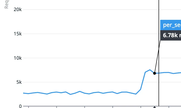
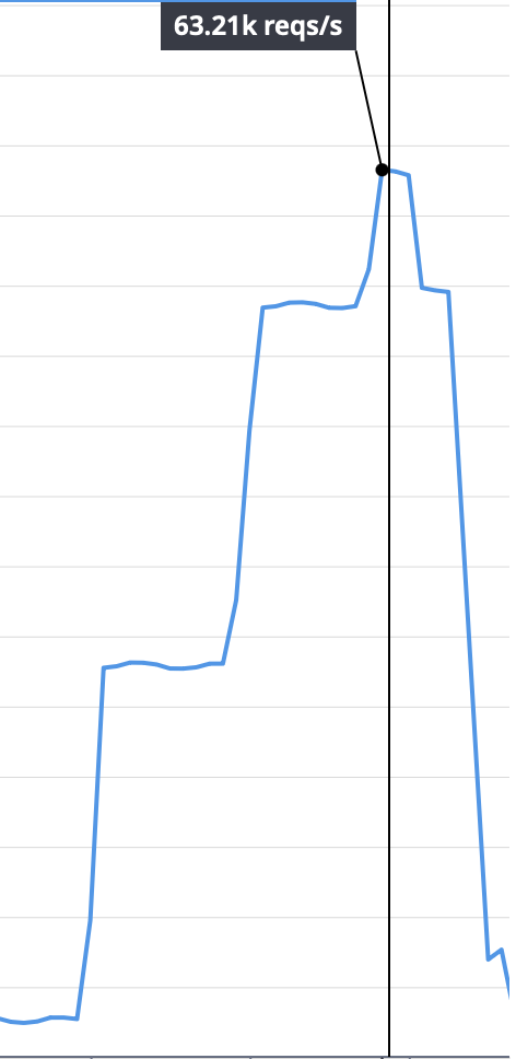
More importantly, another metric that we only tangentially mentioned early on improved as well. When measuring the requests per second handled, we went from ~6000 req/s to 25,000 req/s, a more than 4x improvement in request throughput at minimum. Some benchmark variations allowed us to reach as much as 60,000 req/s, 10x!

All of this while making a good 60–70% use of available CPUs. This is a very good utilisation while leaving some headroom to the soft ceiling of 80%. And since we know the benchmark outlines a worst-case scenario, we are happy to have a capacity buffer of 10–20% of CPU usage on top of the worst-case 🎉

We presented the results to the customer and received many accolades. A job well done.

Conclusion#

First of all, if you are reading this, thank you for bearing with us on this write-up. We hope you learned a thing or two about tuning CouchDB and Erlang. Even if your setup and request load will look very different, you now know how and where to look for bottlenecks.

We also showed that it is important to understand how the whole system works. It allows you to develop a gut instinct for what the most likely candidate for a bottleneck is. This can save you valuable time in a pinch. Of course you must always back up a hunch with data, so don’t skimp on collecting metrics. In this case, our original hunch was correct three times (network throughput, request accept speeds and internal messaging buffers), all of which we could not find in one go but needed distinct measurement tooling for.

An aspect we did not get into is perpetual graphing of metrics. We started work on an extensive metrics dashboard for CouchDB on the customer’s Datadog service and for some things the shape of a graph could already tell us whether we were onto something, or not. We’ll be releasing this as open source software when it is ready and we’ll update this section when that’s available.

We also skipped over many many details, so let us know if you have any questions or if we can help you with your CouchDB performance issue. We also offer a CouchDB monitoring tool called Opservatory that can keep an eye on some of these things for you, and provide some suggestions to get them solved.

If you need help with performance work on your…

• Apache CouchDB,
• Erlang Service,
• Generic Unix Network Service

…book a call today

Take care 👋

« Back to the blog post overview